Established theory is timeless, but many amateurs do not have acces to the archives that contain clasical data of present-day interest. Medium frequency DXers should appreciate this update on an historical 1922 QST article. 1
By H. H. Beverage, ex W2BML* and Doug De Maw, W1FB**
* silent key January 27, 1993
** silent key September 28, 1997
first published in QST (ARRL), January 1982, pp. 11-17
Why the Beverage or “wave” antenna? That’s a question the seasoned 160-meter DXers need not ask, for many of them have used Beverage antennas to enhance the effective signal-to-noise ratio while attempting to extract weak signal from the sometimes high levels of atmospheric noise and QRM. Alternative antenna systems have been developed and used over the years, such as loops and long spans of unterminated wire on or slightly above the ground, but nothing seems to surpass the Beverage antenna for 160-meter weak-signal reception.
The practical limitation for many amateurs is the size of their property: Beverage antenna must be a wavelenght or greater in dimension, which for 160-meter work requires a minimum practical antenna length of 166.6 meters (546.8 feet) at 1.8 MHz (feet = meters x 3.281). In an ideal situation, one would deploy number of Beverage antennas in order to facilitate weak-signal reception from variety of favored directions, such as Europe, South America, Africa and Oceania. The magnitude of the property-size requirements for such a system might seem incomprehensive to the urban amateur but the objective can be and frequently is realized by amateurs who live in rural areas. Some amateurs are part-time users of Beverage antennas.
References appear at the bottom of this article.
That is, they erect one or more of these antennas for short periods of time (with the kind permission of neighbors), mainly to improve reception during 160 meter contests and DX operations. One well known DXer has for many years stretched a Beverage antenna across and beyond an interstate highway (not recommended) for use during 160-meter contest weekends.
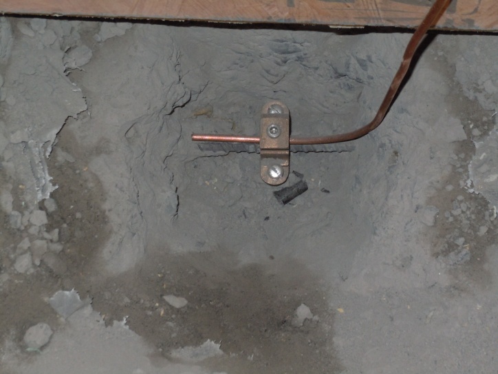
The property requiremens are complicated further by the need for an effective ground system at the terminated end of the wave antenna. Although the ground screen or radials are normally buried a few inches below the surface of the earth, one cannot, without permission, bury a groud system on someone else’s property. Some amateurs have reported reasonable success by driving a number of roos into ground near the terminating resistor, then bonding the rods to one another by means of heavy conductive strap. However, the characteristiss of the antenna are subject to change with the season in accordance with the conductivity of the soil, which is determined in part by the moisture content. The same is true, but to a lesser extent, when buried radials are employed for the ground screen.
Numerous attempts have been made to develop short or “baby Beverages,” but the performance was always a compromise to that of a full size Wave Antenna 2. It is recognized, however, that some improvement in mf weak-signal reception is better than none, so the shortened version of a Beverage antenna may be worth investigation by those who have limited property.
It is ironic that arrays of small receiving antennas, operated in phase and simultaneously rotatable, have been proven to be slightly effective in medium- and low-frequency weak-signal reception. But these arrays also require considerable property if they are to be utilized correctly. Furthermore the cost of such a system, as opposed to a Beverage antenna, is substantially greater.
There seems to be a popular misconception about the frequencies for which the Beverage can provide the stated performance. It is not a suitable antenna for high-frequency reception. One must follow the general rule that applies to loop antennas: employ the Beverage antenna at frequencies and lower. Although some have reported improved reception from Beverage antennas at 3.5 and even 7.0 MHz, the suggested upper frequency limit is 2.0 MHz. Occasional improved reception at hf may result from propagation conditions at a given time, but because the incoming sky waves above medium frequency arrive at moderate and high angles, and with changing polarity because of being reflected from the ionosphere, the Beverage is not suited to effective use in that part of the spectrum.
The wave antenna is responsive mostly to incoming waves of low angle – those that tend to follow the contour of the earth and maintain a constant polarization. This reasoning is applicable to loop antennas as well. The apparent effectiveness of Beverage antennas above 2.0 MHz probably results from a reduction in local QRN and QRM off the sides and back of the antenna. A loop antenna would provide a similar improvement in reception, especially if a sense antenna were included to ensure a cardioid response.
The successful deployment of a Beverage antenna is dependent in part on understanding the concept and development of the system. The following text has been taken from the original disclosure in the amateur literature, which appeared under the H. H. Beverage byline in November 1922 QST. With the recent return of the 1.8- to 2.0-MHz band to U.S. amateurs, and with the easing of the earlier power restrictions in that band, it seems timely to present the original paper again.
Theory and Development
The Wave Antenna, which later became known as the Beverage Antenna, is a unidirectional antenna. It was developed by author H. H. Beverage, Chester Rice and E. W. Kellogg of the General Electric Co., and is covered by patents and applications. The Wave Antenna was first brought to the attention of the amateurs by Paul F. Godley, who described it in his report on the reception of American amateurs at Ardrossan, Scotland.
Theory
If a wire is suspended in space, it has a certain capacitance and inductance per unit length, which bear a definite relation to each other. This relation may be expressed as
![]()
where V is a constant. This constant is the velocity of light. For example, if L and C are expressed as the capacitance and inductance per meter, then V = 3 x 10 meters, which is the velocity of light in meters per second. If a larger wire is used, or if two or more wires are used instead of one, in the ideal case the inductance decreases in the same ratio as the capacitance increases, so that L x C is always a constant. This means that, for the ideal wire, the currents induced in that wire will always travel along it at the velocity of light, independent of the size or number of wires.
A Beverage Antenna needs to be supported at several points and must run horizontally within a few feet of the earth. The effect of the supporting insulators and the proximity of the earth to increase the capacitance in a greater ratio than the inductance decreases, so the velocity of the currents on a practical wire is always somewhat less than the velocity of light. On short wavelengths, however, the velocity approaches very close to the velocity of light, generally between the limits of 85% and 98% of the velocity of light for 200 meters (1.5 MHz), depending upon the size and number of wires.
Fig. 1 – The simplest form of Wave Antenna.
In Fig. 1 is shown the simplest form of Wave Antenna. It consists simply of a wire, at least one wavelength long, stretched in the direction of the transmitting station. For explanation purposes, it may be assumed that the transmitting station is east of the receiving station, and that the receiver is placed at the west end of the antenna, as shown. The traveling wave from the transmitting station moves from east toward the west at the velocity of light. As the wave moves along the antenna, it induces currents in the wire that travel in both directions. The current that travels east moves against the motion of the wave and builds down to practically zero if the antenna is one wavelength long. The currents that travel west, however, travel along the wire with practically the velocity of light, and, therefore, move along with the wave in space. The current increments all add up in phase at the west end, producing a strong signal as shown by curve A in Fig. 2. In a like manner, static or interference originating in the west will build up to a maximum at the east end of the antenna as shown by curve B in Fig. 2.
Fig. 2 – Curve A shows how the current increments add in phase at the west end of the antenna. Curve B illustrates how the static and interference add at the east end of the antenna (see text).
The value of the surge impedance depends upon the size, number and height of the wires above ground, but is independent of the length of the wire. For practical construction with one or two no. 12 copper wires, the surge impedance lies between 200 and 400 ohms. The surge impedance is theoretically equal to
![]()
where L and C are the inductance and capacitance per unit length.
Fig. 3 – Directivity pattern of a Beverage antenna that is one wavelength long. It does not have a damping impedance included.
If the east end of the antenna were open or grounded through zero resistance, all of the energy represented by curve B would be reflected and would travel back over the antenna to the west end, where part of the energy would pass to earth through the receiver and part would be reflected again, depending upon the impedance of the receiver input circuit. The horizontal plane intensity diagram would be bi-directional, as shown in Fig. 3. The reception from the west is not as good as from the east because some of the energy is lost because of attenuation in the wire as the reflected wave travels back from east to west.
Fig. 4 – Directivity pattern to the antenna of Fig 3. The antenna has been damped properly.
In order to make the antenna unidirectional, it is necessary to stop the reflections at the end farthest from the receiver end. This is accomplished simply by placing a noninductive resistance between the antenna and ground at the far end. If this resistance is made equal to the surge impedance of the wire, it absorbs all of the energy and prevents any of it from being reflected back to the receiver. The intensity characteristic becomes unidirectional, as shown in Fig, 4.
Godley used the simple form of wave antenna shown in Fig. 1. However, this is not the most practical form, as it is necessary to go to the far end to make adjustments of the damping resistance.
Feedback Antenna
If two parallel wires are used, the Wave Antenna becames very flexible, and the receiver may be placed at either end with local control of the damping. In Fig. 5, for reception from the east, the receiver at the west end is replaced by the primary, P, of transformer T2. The primary is coupled to the secondary, S, as closely as possible, and feeds the energy over two wires as a transmission line. A second transformer, T1, at the east end, feeds the energy from the transmission line into the receiver. The energy fed over the transmission line circulates around the line as in an ordinary telephone line and, therefore, the currents pass through both halves of the primary of T1 in the same direction, inducing voltages in the secondary, that feed into the receiver. On the other hand, currents coming over the wires as an antenna, that is, from the west, are equal ane in phase on both wires, and upon passing to ground through the two halves of the primary of the output transformer, T1, they pass through the winding in opposite directions and neutralize. With this circuit, the energy reaching the receiver is the same as it would be if the receiver were placed at the west end, except for the transmission-line losses, which ordinarily are 20 to 25% with proper design. With this feedback system the operator can make adjustments of the surge resistance without leaving the station, and can listen to the signals while he or she is making the adjustments.
Fig. 5 – The receiver at the west end of the antenna is replaced here by primary P of T2. (See text)
Fig. 6 is equivalent electrically to Fig. 5, but in this case T2 has been replaced by a simpler circuit. By grounding one wire and leaving the other wire open, the energy is reflected on each wire, but the reflected currents on the transmission line are 180 degrees out of phase on the two wires and, therefore, a difference of potential exists across the terminals of the primary of T1, exactly the same as when the reflection transformer, T2, of Fig. 5 was used. lf the ground resistance at the reflecting end is zero, the reflection of energy with the connections of Fig. 6 would be 100% efficient, and the only loss would be the transmission-line losses. The open ground reflection connection is preferable to a transformer, on short wavelengths particularly.
Fig. 6 – This circuit ia equivalent to that of Fig. 5, except that T2 has been replaced by a simpler circuit. The damping circuit is labeled “D.”
It is possible to damp a two-wire antenna from either end, ln the case of Fig. 6, the signal from the east built up to a maximum at the west end, and was then reflected up to the east end, where the receiver and damping circuit were placed. In the case shown in Fig. 7, the receiver is placed at the west end as in the case of the simple antenna of Fig. 1. Instead of placing the dumping circuit at the east end, however, it is placed across the transmission line at the west end, where the receiver is. This damping circuit is practically just as effective as it would be if actually placed at the far end. This circuit also has the advantage that the desired signals do not pass over the transmission line, and the transmission-line losses are avoided.
Fig. 7 – This example shows the dumping circuit, D, across the two-wire Beverage antenna. The value of the damping resistance will vary with the wavelength.
ln order for the damping circuit to be effective, it is necessary teat the two wires of the antenna be joined through an inductance that is of high impedance compared with the impedance of the damping circuit. The best way to accomplish this result is to use a coil with a midpoint tap as shown at N in Fig. 7. With respect to the transmission line, the two halves of this coil are adding, so the inductance across the line is high. With respect to the receiver, however, the two halves of the coil are opposing, so that the impedance in series with the output transformer amounts only to the leakage reactance of the coil, N, which can be made very srnall. A satisfactory inductor for N, for 200 meters, was a 24-turn coil, 7 inches in diamcter, with a tap at 12 turns for feeding the output transformer, T. This coil was about 0.3 mH across the line, or 1900 ohms at 300 meters (1 MHz), and nearly 3000 ohms at 200 meters, which was high enough to have no appreciable influence on the damping circuit, and yet had low enough leakage reactance to allow the signals to pass to the receiver without noticeable weakening.
Damping Circuits
ln Figs. 6 and 7, damping circuits D are shown that consist af resistance, inductance and capacitance in series. Because of distortion on the antenna, to back-wave effects, to interfering signals or static coming from such a direction as to be received on one of the little “ears” on the back of the antenna, as shown in Fig, 4, and so on, it often happens that there are appreciable residuals that are desirable to eliminate. This is possible by making the damping-circuit reactance either slightly capacitive or slightly inductive, instead of purely resistive. In some cases it may be desirable to reflect a small amount of energy to neutralize undesirable signals from the back end. This is readily accomplished by adjusting the resistance and capacitance of the damping circuit. The capacitance and inductance in this damping circuit are usually found to practically neutralize each other for the best ad justment; that is, they should tune approximately throughout the band of wavelengths it is desired to receive. If the wavelength being received is varied over wide limits, it is necessary to readjust the damping circuit capacitor for best results, although the adjustment is usually quite broad. The resistance does not need readjustment except in special cases.
For a range of 180 to 360 meters (1.66 to 0.83 MHz), the damping circuit consists of an inductance of about 0.08 mH, a variable capacitor of 0.0015 mF maximum capacitance and a noninductive variable resistance in steps of 1 ohm from 0 to 500 ohms. A decade box is ideal for this purpose. However, ordinary wirewound potentiometers (inductively wound), have been used with success in damping circuits. lt is necessary to select a potentiometer with sufficiently low inductance to tune well below the shortest wave it is desired to receive; then the inductance of the potentiometer is taken into account when calculating the value of inductance to be used in series with the resistance and capacitance. In this manner the inductance of the potentiometer used for the variable resistance may be tuned out, and the damping circuit may be made a pure resistance for any one particular wavelength.
When the damping circuit is placed across the transmission line as shown in Fig. 7, the value of the damping resistance may vary considerably with wavelength, becoming lower for short wavelengths, owing to the increase in attenuation at short wavelengths partially damping the antenna. In other words, the transmission liny acts as a resistance in series with the damping circuit, and the transmission-line resistance becomes appreciable at short wavelengths.
Antenna Design
It is obvious from the theory of the Wave Antenna juet given that it most point toward the desired signals or directly away from the desired signals. In case the antenna is pointed away from the signal, then the maximum signal occurs at the far end and must be brought up over the transmission line to the receiver, as shown in Fig. 6. In case the antenna is pointed oward the signal, it is necessary to put the damping circuit on the transmission line, as shown in Fig. 7. It is possible to use a single antenna for reception from either direction by switching arrangements to change to either the connection of Fig. 6, or that of Fig. 7, at will. It is preferable on short wavelengths to point the antenna toward the signal, using the connections of Fig. 7, but the feedback of Fig. 6 gives practically the same results except that the signals are not quite as loud as a result of the transmission-line losses.
It is necessary to run the Wave Antenna in as straight a line as possible and not nearer than 200 feet (61 m) to other parallel wires, such as telephone and power lines, as the influence of these wires is liable to distort the directive characteristic of the antenna. Other wire lines may be crossed at right angles without undesirable effects. ln cases where it is not feasible to run the Wave Antenna in line with the desired signals, it is possible to get good reception with the antenna somewhat “off line” by sacrificing signal intensity. By referring to Fig. 4 it is seen chat for the average antenna one wavelength long, it is possible to be 45 degrees off line before the signal drops to half intensity. Beyond 45 degrees the signal falls off very rapidly. Twenty degrees off line, the signal intensity has fallen off only 10%, so very good reception may be obtained. If the antenna is two wavelengths long, it is more directive, and it is not possible to receive well if it is more than 25 or 30 degrees off line.
The antennas are constructed of copper or other nonmagnetic material, although Cutler of W7IY reported in October 1922 QST that he had obtained good results on a galvanized-iron wire. The size of the wire is usually between no. 10 and no. 14 B&S, although it is possible to get fair results even with no. 18 bell vire. The usual construction is to put up two wires on a cross arm about 2 to 3 feet long. The wires are suspended by porcelain cleats, or in more permanent construction standard telephone pins and high-grade insulators are used.
Fig. 8 – Curves that show the antenna velocity factor as a lunction of the height above ground.
The height of the wires above ground has a marked influence on the velocity of the currents along the wires when the wires are close to the ground, but if the wires are 10 feet above the ground there is little to be gained in velocity by making them higher, as shown in the curves of Fig. 8. These data were taken on an antenna at Belmar, New Jersey, by H. O. Peterson. This antenna extended over fairly conducting soil. The character of the soil underneath the antenna influences the velocity to some extent, but the data of Fig. 8 are about the average velocity. These curves show that the velocity becomes lower at longer wavelengths.
If the velocity is too slow, then the currents in the wire lag in phase behind the wave in space, and a point is soon reached when the current in the wire from the far end is so far behind in phase that it not only does not add to the increments from points close to the receiver, but may actually subtract. The maximum length that it is feasible to use is that length at which the current in the wire lags 90 degrees behind the wave in space. This length is given by
where
l = wavelength in meters
C = signal velocity on antenna, expressed in percent velocity of light
For example, from Fig. 8 we find that the velocity of the currents in the two wires suspended at a height of 10 feet is about 88% of the velocity of light for 200 meters, so the maximum usable length is:
Fig. 9 – Directivity pattern of a Beverge antenna with an effective height of 15 meters, with a vertical or end effect of 3 meters superimposed opon it.
Therefore, it is not feasible to use a two-wire antenna suspended at a height of 10 feet for an antenna that is more than two wavelength long for 200 meters. By increasing the height, the velocity will increase, and longer wires may be used. Fig. 8 shows that the velocity increases slowly with the height about 10 feet, so the wires must be much higher to be of material advantage. Making the wires too high introduces a difficulty on short waves that does not occur on long waves, and that is the “end” or vertical-antenna effect. The effective height of a 200-meter Wave Antenna is about 5% to 10% of its horizontal length, depending upon the nature of the earth beneath the antenna, and so on. If an antenna is 200 meters long, therefore, the effective height will be between 10 and 20 meters. lf the antenna is on supports 10 feet high, the vertical or end effect may be equivalent to an effective height of nearly 3 meters (10 feet), distorting the directive curve. In Fig. 9 is shown the directive curve of a Wave Antenna of 15-meters effective height with a vertical or end effect of 3 meters superimposed upon it. It will be noted that the end effect may mount up to very serious proportions if the antenna is made too hogh. It is, however, possible to balance this end effect by means of a separate vertical antenna, as shown in Fig. 10. P1 is the standard primary, while P2 is a second primary coil of about the same number of turns, which is wound over P1 but in the opposite direction. ln practice, however, the end effects seem to be very much smaller than predicted theoretically, so as a general rule if the antenna is not over 10 feet high the end effects are so small that it is not worth the trouble to balance them. From the foregoing considerations, it is evident that 10 feet is a good average height for short Wave Antennas.
Fig. 10 – A separate vertical antenna can be used to balance out the end effects discussed in the text. The circuit arrangement is depicted here.
Design of Transformers
With the feedback circuit of Fig. 6, only one transformer is necessary. The output transformer, T1, was wound on a 7-inch cardboard tube. The primary, P, was 20 turns of no. 24 enameled copper wire, with a tap at 10 turns or the exact center. Over the primary was placed a shield consisting of a piece of tinfoil insulated from both windings by means of paper. This shield was grounded to cut out capacitive currents between primary and secondary. It is important that the tinfoil or other metal foil be not quite a complete turn around the primary; the ends must not touch or it will act as a shortcircuited turn and introduce high losses. The secondary consisted of 5 turns of no. 18 bell wire wound over the tinfoil shield. The center of the secondary winding was lined up carefully over the center of the primary winding; otherwise the transformer would not be balanced. With the circuit of Fig. 6, the transformer balance was tested by opening both wires at the west or reflection end. When T1 was properly balanced, the receiver was quiet, indicating that the two halves of the primary were perfectly symmetrical with respect to the secondary.
T1 of Fig. 6 was designed to work with a coupled receiver. The secondary of the output transformer was connected in series with the primary winding of the receiver input transformer and was tuned by the series capacitor, C. For 200 meters, it is usually better to use a separate capacitor, C, outside of the tuner capacitor as shown in Fig. 5, but for longer wavelengths this series capacitor may be omitted.
When the circuit of Fig. 7 was used, the transformer just described was used with sucess, but better results were obtained by cutting the primary turns down to 15 instead of 20. This transformer is shown in Fig. 1, but may be used with the connections of Fig. 7. A metal-foil shield is used between primary and secondary, and is grounded as shown. In all of these transformers the coupling between primary and secondary should be as close as possible.
Fig. 7 illustrates an auto-transformer, T. The total turns are 15, and the receiver is tapped off at 5 turns. The diameter of the turns is 7 inches, but smaller diameters have been used by increasing the number of turns to obtain the same inductance. This auto-transformer connection was once adapted to a Reinartz tuner with excellent results by Roland Bourne, W1ANA, at W2BML.
Surge Resistance and Velocity Factor
The velocity factor and surge resistence were easily deterrnined by oscillator tests. An oscillator was coupled to the antenna, as shown in Fig. 11. A coupling coil, L, was included in the antenna circuit. It consisted of only two turns. The far end of the antenna was left open for the first test, and a resonance curve of the antenna was taken. The curve is plotted as curve A in Fig. 12. Then both wires of the antenna were grounded at the far end, and the resonance curve taken again. This is shown as curve B in Fig. 12. In order to find the velocity, it is necessary to calculate what the resonance points would be if the velocity of the currents on the wires were equal to the velocity of light.
Fig. 11 – An oscillator can be coupled to the antenna, as shown here, to determine the veloclty factor and surge resistance.
The length of the antenna was carefully measured. In the case of this particular antenna at Belmar, New Jersey, the length was 240 meters. Assuming that the velocity of the currents on the antenna is equal to the velocity of light, the first resonance point with the far end of the antenna open will be the quarter-wave oscillation, as in an ordinary antenna. The wavelength will be 4 x 240 = 960 meters. The next resonance point will be the three-quarterwave oscillation, or 4/3 x 240 = 320 meters. The next will be the 5/4 oscillation, or 4/5 x 240 = 192 meters, and so forth, for all odd multiples of the quarter-wave oscillation. ln a like manner, with the far end of the antenna grounded, the antenna will oscillate at all even multiples of the quarter-wave oscillation. These calculated values are recorded in Table 1. In the next column, the observed values taken from Fig. 12 are recorded. By dividing the calculated value by the observed value, we get the actual velocity at that particular wavelength in terms of percent of velocity of light.
Fig. 12 – Curves obtained with oscillator tests of a 240-meter long Beverage antenna (see text).
Table 1.
Calculation of Velocity of Currents on Antenna
Length – 240 meters, 2 no. 10 wires, 3 meters high
| Mode of Oscillation | Wavelength Calculated | Wavelength Observed | Vel/Wires Vel/Light |
| 1/4 | 960 | 1200 | 80% |
| 2/4 | 480 | 590 | 81% |
| 3/4 | 320 | 390 | 82% |
| 4/4 | 240 | 280 | 86% |
| 5/4 | 192 | 220 | 87% |
| 6/4 | 160 | 180 | 89% |
To determine the surge resistance, a noninductive resistance was placed between antenna and ground at the far end, and the resonance curve was taken again. Fig. 13 shows the results of the test on the Belmar antenna. Curve A, with 500 ohms at the far end, shows broad but remarkable resonance points at open oscillation wavelengths. On the other hand, curve B, with 200 ohms at the far end, shows grounded resonance points. Curve C, with 300 ohms at the far end, shows no resonance points, indicating that the antenna is quite aperiodic. Therefore the surge resistance for this particular antenna is approximately 300 ohms. The downward bend of curve C below 200 meters is not caused by the antenna, but results from the oscillator output falling off when the coupling capacitor approached zero setting.
When one of the wires was grounded at the far end, the other wire was left open and the damping resistance was placed across the wires at the station end, as shown in Fig. 7, a smooth curve, similar to the curve C of Fig. 13, was obtained when the noninductive resistance was 500 ohms. In this case, however, there were slight irregularities in the curve that do not appear in curve C of Fig. 13.
Flg. 13 – Damping curves for a two-wire Beverage antenna (see text).
Fig. 14 shows the resonance and damping curves taken on a single-wire antenna by R. B. Bourne at W2BML/W2EH. This wire was 195 meters long, and was suspended from trees at a height varying from 15 to 20 feet. It was interesting to note that Bourne’s antenna had a velocity of approximately 93% of the velocity of light at 200 meters and, therefore, showed that a single wire could be used up to a length of over three wavelengths, or approaimately 2000 feet. Such an antenna should show very directional properties, but lacks the flexibility and ease of adjustment of the two-wire antenna.
Fig. 14 – Damping curves for a single-wire Beverage antenna.
Performance
Two 200-meter Wave Antennas were erected at Belmar, one running west from the station and the other running south. These antennas were arranged with switching such that the connections of Fig. 6 or Fig. 7 could be selected at will on either antenna. That is, the west antenna could be used for reception from either the east or the west, and the south antenna could be used fot reception from either the north or south. For comparative purposes a flat-topped single-wire antenna, 40 feet high, was erected. The effective height of this vertical antenna was estimated as approximately 8 meters. The signals on the Wave Antennas were about 50% stronger than on the vertical, giving an effective height for the Wave Antennas of 12 meters. This figure corresponds to about 5-1/2% of the horizontal length of the Wave Antennas.
Listening tests on these antennas showed marked directive properties, as expected. Listening south, most of the stations heard were in the third and fourth districts, but careful adjustments were nwcessary to eliminate second-district stations to the north. With the antenna directive toward the north, the best reception was from the first and second districts, although several eighth-district stations were heard. The east-west antenna worked better than the north-south antenna, probably because the ground resistance at both ends was less than an ohm, whereas the ground resistance at the far end of the north-south antenna was very high (nearly 300 ohms) making it difficult to operate the damping circuit effectively. The reception from the west was excellent, great numbers of Midwest, Southwest and West Coast cw staticrns being heard without interference from first- and second-district stations. With the antenna directed east, only local W2s, Long lsland W2s and a few W1s were heard. There was considerable QRN reduction at times on the eastward reception, as the QRN was often heavy in the south or west.
On the 360-meter broadcast station wavelength, very good results were experienced in eliminating interference, particularly when using the antenna for west reception and cutting out New York and Schenectady interference. Station WOC at Davenport, Iowa, was received particularly well on the Wave Antenna at times when reception was impossible on the vertical antenna, owing to local interference.
Even on 600 meters, these Wave Antennas showed very good directivity, particularly for reception from ships at sea.
Bourne’s antenna at Riverhead, Long Island, ran in a direction about 10 degrees north of west. He reported his results as follows: “Signals from the south and southwest come in with about 25% to 50% increase in signal strength over a vertical antenna 60 feet high. Signals from New England are, in general, very weak, and in some cases cannot be heard at all when using the Wave Antenna. No interference from ships or shore stations using commercial wavelengths was noticed. WSA, at Easthampton about 20 miles away, at times had a very strong harmonic on about 225 meters, which interfered seriously with 200-meter reception when the ordinary antenna was used, but because this station was southeast, no interference was experienced when using the Wave Antenna. Radiophones on 360 meters came in with about the same intensity as with the vertical antenna, but often the signal-static ratio was much improved with the Wave Antenna, and, as with 200-meter reception, interference from WSA and WBC (East Moriches, 10 miles away) was entirely done away with.”
The amount of static reduction experienced with the 200-meter Wave Antenna at Belmar depended entirely upon the distribution of the static at different times. On several occasions a marked improvement was noted in the signal-static ratio when receiving from the east and north, and sometimes when receiving from the west, but it was rarely observed to make any marked improvement when receiving from the south.
The author wishes to acknowledge the valuable assistance received from Messrs. H. O. Peterson, R. B. Bourne and A. B. Moulton, in the collection of these data on the 200-meter Wave Antennas.
Practical Considerations
The foregoing text from the 1922 QST article discusses slight differences in overall performance with respect to the wire gauge used in a wave antenna, with the smaller-diameter wire being the less desirable choice. In a practical amateur installation it is unlikely that one could discern a performance difference without having two antennas to compare – one with heavy-gauge wire and one with, say, no. 20 wire. Many amateurs have reported good results when using the smaller wire sizes for single-wire Beverage antennas. But, if the heavier wire is available, it should be employed in the interest of optimum performance. The longevity of the system under the stresses of wind and icing will be superior when the antenna is made from no. 10 through no. 16 wire. If for some reason it is desired to have a measure of “invisibility” for the antenna, one should not overlook the possibility of using light-gauge wire.
Quality insulators are required at the support points of the wire. Some amateurs have merely secured their Beverage antennas along the span by wrapping the conductor around tree trunks and fence posts. This is not recommended if proper performance is desired. The incoming signal energy should be able to traverse the wire without propagation discontinuities and losses along the antenna length. Good insulators will help to make this possible.
The least complex of the Beverage antennas is the single-wire version, although the two-wire type offers greater flexibility of adjustment. In any event, the integrity of the termination and ground system is a matter of prime importance. Some amateurs have simply driven an 8-foot pipe into the ground at the far end of the antenna, then attached the terminating resistor to it. Depending upon the earth conductivity at a given location, this technique may represent no ground system whatsoeverl A quality ground system contains a substantial number of buried radial wires, as is the case with quarter-wavelength vertical antennas. If an extensive ground arrangement isn’t practical, the amateur should use as much wire as possible, even if some of the radials are quite short. Sufficient wire should be used to ensure that the ground resistance is as low as possible.
Other Considerations
Fig. 15 illustrates a Beverage antenna used by W1FB (then W8HHS) in Michigan for 160-meter reception in the early 1950s. It was roughly 1500 feet (three wavelengths) long, which posed no physical problems on the 40-acre farm site. The terminated end was toward the northeast to accommodate reception from Europe. The transmitting antenna was a 60-foot vertical with center loading and 20 buried radials that were dispersed uniformly from the base of the vertical to a length of 80 feet each. Signals that could not be heard in the noise while receiving with the vertical could be elevated above the atmospheric noise by as much as two S units when using the Beverage antenna for DX work to Europe. Owing to the majority of the noise fronts existing to the southwest, in the Gulf of Mexico region, and because of the back-rejection of the Beverage, such an improvement was possible. Heavy QRN could often be heard with the vertical, even though the weather was clear locally and for a thousand miles or more to the southwest. Noise from storms can be propagated a great distance when conditions are other wise good at 1.8 MHz.
Fig.15 – Circuit of the 160-meter Beverage antenna used at W8HHS for DXreception. The primary and secondary windings of T1 were returned toseparate ground points to resotve unwanted common-mode bc-bandsignal coupling that affected receiver performance.
One problem that was experienced with the antenna of Fig. 15 became manifest as severe receiver overloading from a nearby commercial a-m station on 1240 kHz. The receiver dynamic range and front-end selectivity of that period were generally anything but spectacular. Hence, crossmodulation and other overload effects were not uncommon to 160-meter operators. The difficulty was resolved by breaking up the common-mode transfer path from the antenna to the receiver. At first the return ends of the primary and secondary windings of T1 were brought a common ground point. By returning the low end of the T1 primary to the receiver ground terminal and the low end of the secondary to the earth ground, the overloading ceased. The Beverage antenna was an effective collector of bc-band energy! T1 was used to provide a broadband transformation from 300 ohms (unbalanced) to 50 ohms unbalanced at the receiver input. A small TV-set flyback transformer core was used in the transformer. A 900 mi ferrite toroid core would be excellent for the purpose today.
References
1 H. H. Beverage, “A Wave Antenna for 200-Meter Reception,” QST, November 1922, p. 7. The professional disclosure of the wave antenna was presented by H. Beverage, C. Rice and E. Kellogg (“The Wave Antenna, a Ncw Type of Highly Directive Array”), in the Transactions of the AIEE for 1923. It contains 51 pagcs of technical information.
This presentation of the original QST work by Beverage has been edited for style, tense and terminology to bring it up to present-day QST technical language. The diagrams, curves and radiation patterns have been redrafted to conform to presentday symbology and style. Nothing else has been changed. The reprint of the article is presented in smaller type size to differentiate between the writing of H. H. Beverage and D. DeMaw.
2 B. Boothe, W9UCW, “Weak Signal Reception at 160 – Some Antenna Notes,” June 1977 QST.
3 J. Reinartz, W1QP, “Some Further Improvements in My Tuner,” QST, October 1921, p. 12.
