A revolutionary addition to the LF band segment.
The principal problem of any LF antenna is its dependence on the ground properties. A low angle radiation is the mandatory, therefore an usual horizontally polarized antenna is useless ifnot located a half wavelength above the ground (i.e. 40 or 80 meters for 80 or 160 m band respectively). Vertical monopoles are better but the major disadvantage is the need of an extensive mesh of radials. A low profile ground-independent radiator would be a suitable solution. It is the Gieskieng antenna.
This antenna is a result of experimental work of D. H. Gieskieng, W0FK. The first look says that it is no wonder antenna but specially shaped vertical dipole. This is not true, better explanation brought the co-inventor, Harold Aspden of Southampton University.
“In summary, the Gieskieng antenna differs from conventional antennas in that it is expressly designed so that the electric field energy and the magnetic field energy are not forced into the field medium in time-phase with each other, as applies for a conventional half-wave dipole. Instead, the antenna is so structured that the electric and magnetic fields are set up in quadrature phase. For the same excitation this appears to produce a signal of half strength initially, but it has, it seems, the property of being less subject to dissipation and attenuates more in accord with theoretical prediction, whereas conventionally produced signals attentuate more rapidly.
It will be argued that this phenomenon is attributable to the field medium having a natural propagation mode which is directly excited by the Gieskieng antenna, whereas the excitation by the dipole antenna develops a forced propagation mode with which we are familiar, the forced propagation degenerating into natural mode propagation with energy dissipation over an initial range of transmission.”
For those interested in more thorough theoretical background I highly recommend both articles describing the antenna evolution, testing and results.
These articles are at
http://www.aetherscience.org/www-energyscience-org-uk/feedback/fn03.htm (D. H. Gieskieng) and
http://www.aetherscience.org/www-energyscience-org-uk/le/le10app.htm (H. Aspden).
This antenna can be used as a separate radiator as well as the part of more complex arrays (four square etc.). The Gieskieng antenna exhibits many interesting advantages:
It is not a fiction of an ideal antenna, because:
- it is narrow band antenna (in spite of SWR), the SWR = 2 bandwidth on 1.8 MHz is about 20 kHz, on 28 MHz about 250 kHz)
- it is a monoband antenna
- two support poles (trees) needed
Description
The mathematical model was analyzed with the NEC2 system (4NEC2D).The original antenna by D. H. Gieskieng has both horizontal parts of the same length and is constructed as “quite” thick radiator (Fig. 1) with both horizontal parts of 0.215 l, vertical part of 0.0574 l and the radiator diameter of 0.0047 l.
Fig. 1. The original GIESKIENG antenna.
The modified antenna (Fig. 2) is made of wire, therefore the vertical part was splitted to two sloped halves. The construction was optimized for each band for best SWR and radiation angle. The different length of both horizontal parts is a result of optimization procedures.
 Fig. 2. The modified GIESKIENG antenna.
| Freq. |
A |
B |
C |
D |
E |
F* |
| [MHz] |
[m] |
[m] |
[m] |
[m] |
[m] |
[m] |
| Wavelength |
0.19 |
0.24 |
0.064 |
0.04 |
0.1 |
0.11 |
| 1.825 |
31.51 |
40.48 |
10.20 |
6.56 |
15.62 |
3.0 |
| 3.525 |
16.31 |
20.96 |
5.28 |
3.40 |
8.08 |
3.0 |
| 5.373 |
12.29 |
12.29 |
3.4 |
2.2 |
5.2 |
3.0 |
| 7.010 |
8.20 |
10.40 |
2.65 |
1.71 |
4.06 |
3.0 |
| 10.110 |
5.69 |
7.20 |
1.84 |
1.18 |
2.82 |
3.0 |
| 14.050 |
4.10 |
5.22 |
1.32 |
0.85 |
2.02 |
2.0 |
| 18.080 |
3.20 |
4.06 |
1.03 |
0.66 |
1.58 |
2.0 |
| 21.050 |
2.74 |
3.48 |
0.88 |
0.57 |
1.36 |
1.7 |
| 24.900 |
2.32 |
2.95 |
0.75 |
0.48 |
1.14 |
1.5 |
| 28.050 |
2.06 |
2.61 |
0.66 |
0.43 |
1.02 |
1.0 |
* lowest wire above the ground.
The lower horizontal wire is stretched at 0.11 λ above the ground (18.74 m or 61 ft. for 160 m). The model was shifted around the Z axis to change the height above ground and the SWR, radiation pattern and wave angle was observed. The antenna showed excellent properties from 3(!) to 19 meters above the ground.
WARNING! This (and many other) antenna won’t work properly unless an efficient RF choke (balun) providing choking impedance Z>4 kΩ is used. The feeder MUST BE ISOLATED from the radiator, see http://www.karinya.net/g3txq/chokes/.
Use purely resistive choke, reactive chokes are undesirable!
Antenna modeling notes:
The Gieskieng antenna was modeled above realground using the Sommerfeld-Norton approximation with a single planar homogenous medium:
FINITE GROUND.
SOMMERFELD SOLUTION
RELATIVE DIELECTRIC CONST.= 13.000
CONDUCTIVITY= 5.000E-03 MHOS/METER
COMPLEX DIELECTRIC CONSTANT= 1.30000E+01-6.39716E+00
which represents anaverage ground (pastoral, medium hills and forestation, heavy clay soils).
The observed structure has 105 elements. Symbolic SY “cards” are specific for the 4NEC2D software, here enabled the optimizing procedures.
CM 160 m GIESKIENG Antenna
CM Created on 07-jan-03 by OK1RR
CE
SY x1=-6.56
SY x2 = 31.512
SY x3 = 40.481
SY z1=3
SY z2=z1+7.81
SY z3=z1+15.62
GW 1 21 0 0 z1 x3 0 z1 #12
GW 2 21 0 0 z1 0 0 z3 #12
GW 3 21 0 0 z1 x1 0 z2 #12
GW 4 21 x1 0 z2 0 0 z3 #12
GW 5 21 0 0 z3 x2 0 z3 #12
GE1
EX 0 2 11 00 1.0 0.0
GN 2 0 0 0 13 .005
FR 0 1 0 0 1.825
EN
Very interesting is a comparison of GIESKIENG antenna 3 m the ground and an Inverted Vee with apex at 20 m (Fig. 3). The radiation of the GIESKIENG antenna is flat with a low angle which ensures good results for DX work. Inverted Vee radiates perpendicularly at 90 degrees which is good only for local QSO.
Fig. 3. A comparison of vertical radiation pattern of GIESKIENG antenna
3 m above the groundand an Inverted Vee with apex at 20 m.
Fig. 4. shows vertical radiation angle vs. antenna height (lowest horizontal wire).
Fig. 4. Vertical radiation angle vs. antenna height.
The pattern shows a slightly better suppression of high angle radiation at some heights but the radiation angle itself is quite independent on the antenna height and is about 30 degrees. The Gieskieng antenna retains its good properties also in low heights above the ground. If you want to model this antenna with a MININEC based program (i.e. MMANA by JE3HHT), reckon all limitations of this method. MININEC based programs offering rather less accurate results if the analyzed structure contains wires at 0.2 Ã}» above the ground or less, similar problem may occur with parallel wires.
Commercially available ELNEC by W7EL and many other programs have built-in correction algorithm. MININEC itself is limited to 256 segments, you may encounter some problems with “real world” structures above defined ground.
The Sommerfeld-Norton approximation used here works only with with NEC-2 engine and also with NEC-3 and NEC-4, for which is needed a special license from Livermore Institute.
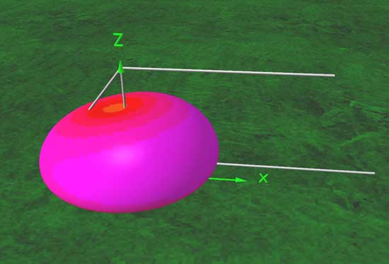
Practical results of MININEC method are useful at structures up to 256 segments, so can be used here. Some cumulated inaccuracies may occur if a MININEC based optimizer is used (impedance circumstances or field intensity at the near/far field zone border etc.). The following 3D radiation pattern model (far field) of the GIESKIENG antenna was created with the NEC-2 (4NEC2D) program using Sommerfeld-Norton ground approximation.
Fig. 5. 3D radiation pattern model (far field).
Fig. 6. shows the near field pattern. The blue level pouring to infinite represents lowest intensity levels.
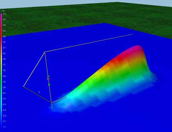
Fig. 6. 3D radiation pattern model (near field).
Impedance pattern
The GIESKIENG antenna is quite narrow band in spite of SWR (for SWR = 2 shows on 160 m a bandwidth of 20 kHz, on 10 m some 250 kHz). The radiation pattern is less frequency dependent.
Fig. 7. SWR and reflection coefficient.
Both drawings showing low SWR bandwidth (a deep narrow resonance dip, Fig.7). The antenna should be tuned by length varying (cutting) of the lower horizontal wire. If you plan to use the GIESKIENG antenna as a part of phased arrays (i.e. four square), all elements should have the same impedance vs. frequency relationships which is not quite easy to obtain. A Smith chart representation of impedance vs. frequency shows Fig. 8. Note the steep rise of reactive component if the frequency changes from 1825 kHz to both directions (antenna with lower horizontal wire at 18.74 m, total height 34.36 m). If the antenna is lowered to 3 m, there is less advantageous behaviour (SWR min. 1.7).
Fig. 8. A Smith Chart representation of impedance vs. frequency.
Antenna construction
Two supports are needed. A pipe mast can be used for the main radiator if the tubing is split with insulators to three parts (Fig.9). First insulator separates the antenna from the supporting part, the second one is placed at the feed point. Both sloped parts are made of wire, the triangle vertex is held in its position with a guy rope. The lower horizontal wire is equipped with a pigtail for easy tuning, it can be easy cut to lowest SWR on desired frequency.
Fig. 9. Antenna construction
You can misuse a nearby tree or a pole as the second support. There is no need of insulators if a good isolating rope is used. The precalculated dimensions of the GIESKIENG antenna for all HF bands shows the table. The row marked with l means dimensions in wavelengths. The dimension F (asterisk marked) is the antenna height above ground which should be 0.11 l for best SWR. 160 and 80 m values are minimal without any noticeable deterioration of SWR, bandwidth and radiation angle. As usual, the resonant frequency tends to drop down if the antenna height is lowered, the antenna at 3 m shows an SWR of 1.7 with A = 31.27 m and B = 39.83 m.The antenna was modeled with #12 wire (2,053 mm) but the wire diameter is less critical. The initial tests were made on the 2 m band.